How to Use CHITRA

HOW TO USE CHITRA?

Below are the step-by-step instructions, accompanied by pictorial representations, to ensure a seamless experience with CHITRA.

Step 1: Getting Started

• On the landing page, click the “Get Started” button to begin.

Step 2: Uploading Files or Viewing Example Data

• On the next page, you can either:

1. Upload Files
2. View Example Datasets

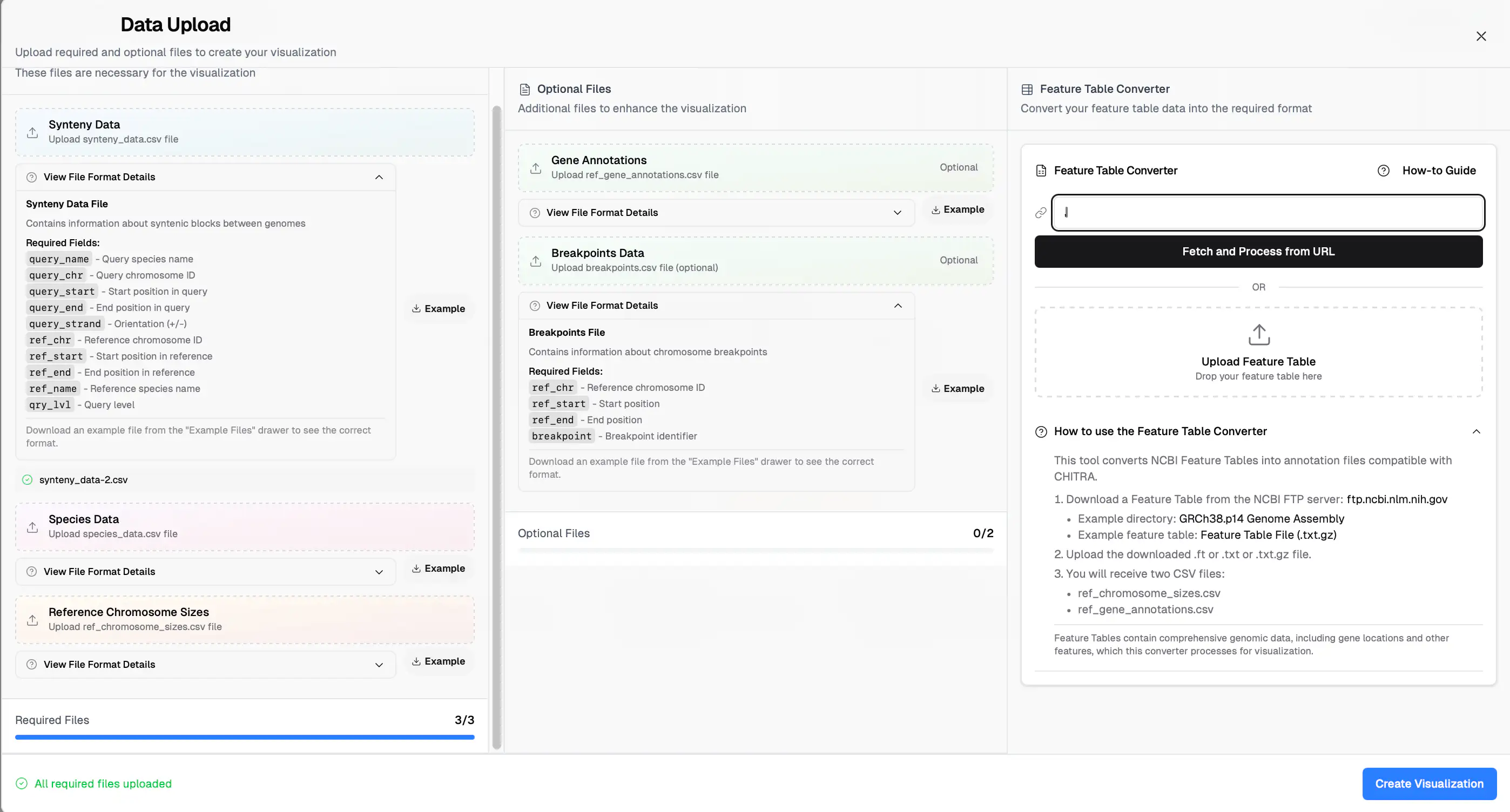
2.1.1 File Upload Instructions

Mandatory Input Files:

1. Synteny Data
2. Genome Data
3. Reference Chromosome Size

Optional Input Files:

1. Gene Annotations
2. Breakpoint Data

To upload files:

Click the “Upload Data” button. A popup window will appear where you can browse and upload the required input files.

Note: All input files should be in CSV format

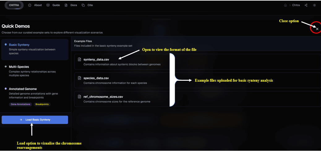
2.1.2 Using Example Datasets

CHITRA includes pre-loaded example datasets to help users explore its functionality. Three types of example datasets are available:

1. Basic Synteny

Visualize synteny blocks among three genomes.

Input files required:

2. Multiple Synteny

Compare synteny blocks among multiple genomes. Uses the same files as Basic Synteny.

3. Annotated Genome

Analyze annotated genomes using real datasets. Uses the same files as Basic Synteny, plus these additional files:

Available Datasets

Three types of example datasets are available:

1. Basic Synteny

• Simple synteny visualization between genome.
• Ideal for understanding the fundamental concepts of synteny blocks and chromosome mapping.

2. Multi-Genome

• Complex synteny relationships across multiple genome.
• Allows comparison of genomic architecture across diverse organisms.
• Includes data for multiple pairwise comparisons.

3. Annotated Genome

• Detailed genome annotations with gene information and breakpoints.
• Includes gene features, locus tags, and symbols.
• Provides breakpoint data for structural variation analysis.

[!NOTE] You can preview and download the example data tables directly from the example files drawer below.

Exploring Example Data

• Select any of the three options in the drawer to access the files.
• You can preview the data or download the files directly.
• Click "Load" to automatically populate the visualization with the selected dataset.

Feature Table Converter

This tool converts NCBI Feature Tables into annotation files compatible with CHITRA.

How to use the Feature Table Converter

1. Download a Feature Table

   • Get the file from the NCBI FTP server.
   • Example directory: GRCh38.p14 Genome Assembly
   • Example file: Feature Table File (.txt.gz)

2. Upload the File

   • Upload the downloaded .ft, .txt, or .txt.gz file to the converter.

3. Download Converted Files

   • You will receive two CSV files compatible with CHITRA:
     • ref_chromosome_sizes.csv: Contains the size of each chromosome.
     • ref_gene_annotations.csv: Contains detailed gene annotation data.

Note: Feature Tables contain comprehensive genomic data, including gene locations and other features, which this converter processes for visualization.

Data Preparation & External Tool Integration

To assist users in transitioning from standard bioinformatics tool outputs to CHITRA, we provide the following mapping guidance.

Mandatory CSV Schema Definitions

Before preparing your data, ensure your CSV files follow these column naming conventions:

Mapping from Popular Synteny Callers

If you are using external tools, map their outputs to CHITRA's schema as follows:

SyntenyTracker2: The Preferred Workflow

For a seamless experience, we recommend SyntenyTracker2 as the companion tool for data preparation. It is designed to modernize modular synteny pipelines and simplify the path to visualization by generating data with exact genomic coordinates.

Installation via Conda:

conda install jitendralab::syntenytracker2

By using SyntenyTracker2, you can generate all mandatory input files for CHITRA in one step, ensuring high reproducibility and significantly reducing the data preparation burden.

Working with MCScanX Data

MCScanX is a popular comparative genomics toolkit used to detect syntenic and collinear gene blocks from raw genome annotation and homology data.

Typical MCScanX Workflow:

1. Generate all-vs-all BLASTP results between your genomes.
2. Prepare a GFF/BED file containing your gene coordinates.
3. Run MCScanX using these inputs to produce a .collinearity file for downstream analysis.

[!WARNING] Important Limitation regarding MCScanX: MCScanX predicts collinearity by connecting individual homologous genes based on e-values (e.g., matching chr1_gene001 to chr3_gene221), rather than exporting the exact start/end boundary coordinates of a contiguous physical DNA block. Since CHITRA currently requires exact boundary mappings (like those produced by Satsuma or SyntenyTracker) to render physical chromosome ribbons, MCScanX .collinearity outputs currently require you to run a custom intermediate script to convert those gene-to-gene links into standard block coordinates before uploading to CHITRA.

Future Support: In a future release, CHITRA plans to directly support parsing .collinearity output files. We intend to automatically infer and group these connected lower-e-value threshold genes to bridge and generate broader syntenic regions between chromosomes directly within the application.

Raw Data Viewer — Column Reference

The Raw Data Viewer (accessible via the View Data button in the toolbar) displays the loaded data across five tabs. Each column header has an inline ℹ tooltip and a Column Guide button per tab. The full definitions are listed below.

[!NOTE] All positional values (start, end, size) are in base pairs (bp) unless stated otherwise. Columns marked (optional) may show N/A if not provided in the input file.

Synteny Table

Displays pairwise synteny block coordinates between the reference and query genomes.

Genome Table

Lists all chromosomes and their sizes for every genome loaded into CHITRA.

[!NOTE] centromere_start and centromere_end are optional. If omitted, chromosomes are drawn as plain rectangular bars without a centromere marker. Providing them enables metacentric/submetacentric chromosome morphology rendering.

Reference Table

Contains size information specifically for the primary reference genome used as the coordinate base.

Genes Table

Gene annotation data for the reference genome (loaded via ref_gene_annotations.csv or the Feature Table Converter).

Breakpoints Table

Chromosomal breakpoint intervals on the reference genome (loaded via breakpoints.csv).